Browse all 47 figures in paper order, with their original captions. Select an image to view it at full size.
Figures by Pierre Guilbert, licensed under CC BY 4.0. Please credit the author and paper when reusing or adapting a figure.
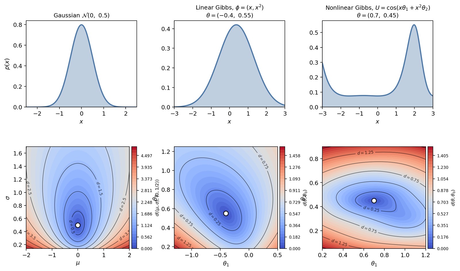
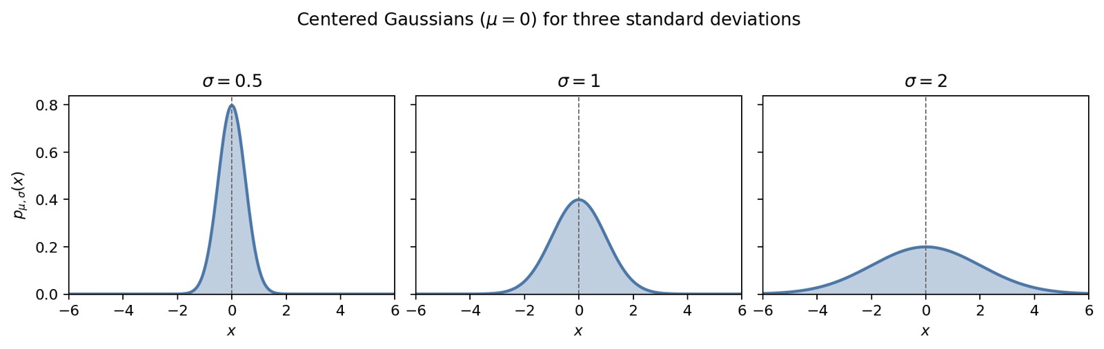
Figure 1. Three univariate parametric families (first row) and
iso-contours in the parameter plane (second row). Left column: exact
Fisher–Rao distance around
.
Middle and right columns: Riemannian length of the Euclidean chord (an
upper bound on the geodesic distance), for the linear Gibbs family
and the nonlinear Gibbs family
.
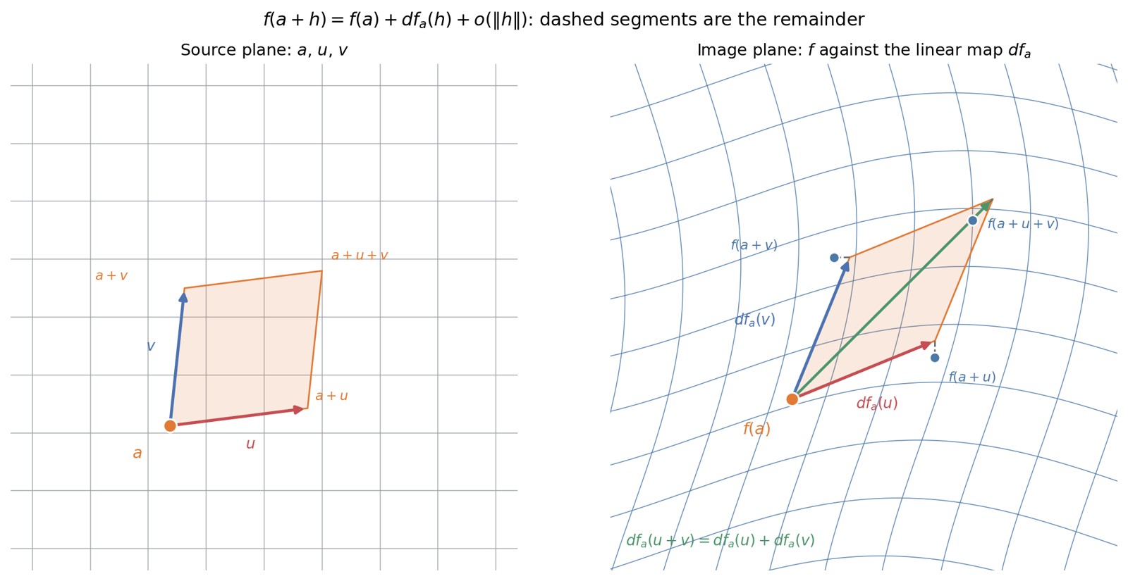
Figure 2. The Fréchet differential of
at the point
.
Left: the Cartesian grid of the source plane, the base point
,
the two vectors
and
,
and the parallelogram they span. Right: the same grid transported by
,
which curves it, together with the images
,
and
of the three other vertices. Superimposed at
is the parallelogram generated by
and
:
the linear map
preserves the parallelogram structure, and its diagonal is
.
The dashed segments measure the distance between the linear model and
the true images; they are the remainder
,
and they shrink faster than
as
and
are shortened.
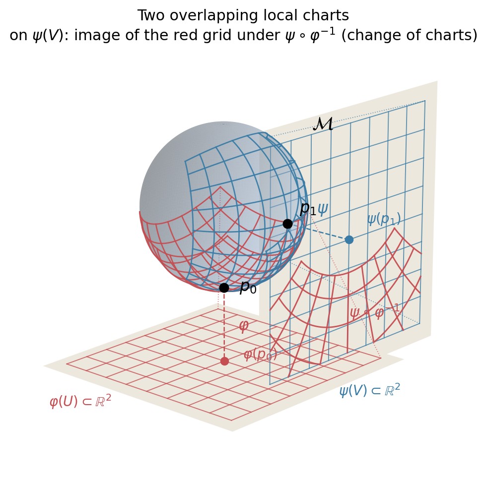
Figure 3. Two overlapping local charts. Here
is the sphere,
its south pole, and
its east pole. The chart
(red) maps a neighbourhood of
onto the lower plane; the chart
(blue) maps a neighbourhood of
onto the plane on the right. The two grids, pushed onto
by the inverse maps, intersect. In the blue plane, the deformed red grid
is the image of this overlap under
:
the transition map remains smooth.
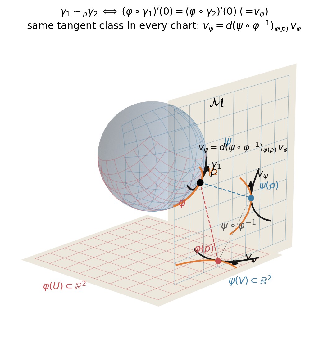
Figure 4. Intrinsic definition of a tangent vector as an equivalence
class of curves. On the manifold
,
the curves
(black) and
(orange) both pass through
with the same velocity but different curvature. In each chart their
images remain distinct, yet they share a common tangent arrow at the
chart image of
:
and
.
The transition map
relates the two representatives by
,
which is precisely the chart-independence of the equivalence relation
.
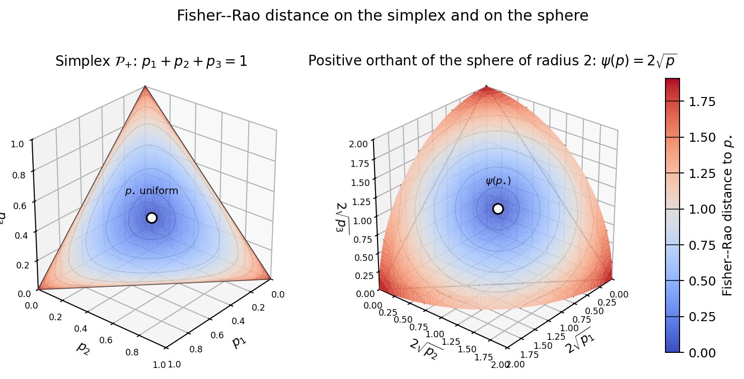
Figure 5. Effect of the embedding
on the metric. On the left, the simplex
of densities
with
;
on the right, its image under
,
the positive orthant of the sphere of radius
.
Both surfaces are coloured by the Fisher–Rao distance to the uniform
distribution
,
marked in white, together with its iso-distance curves. On the right,
these are the geodesic circles of the sphere; on the left, their images
under
.
These curves become denser near the boundary of the simplex: one of the
coefficients
approaches
,
and the metric
diverges.
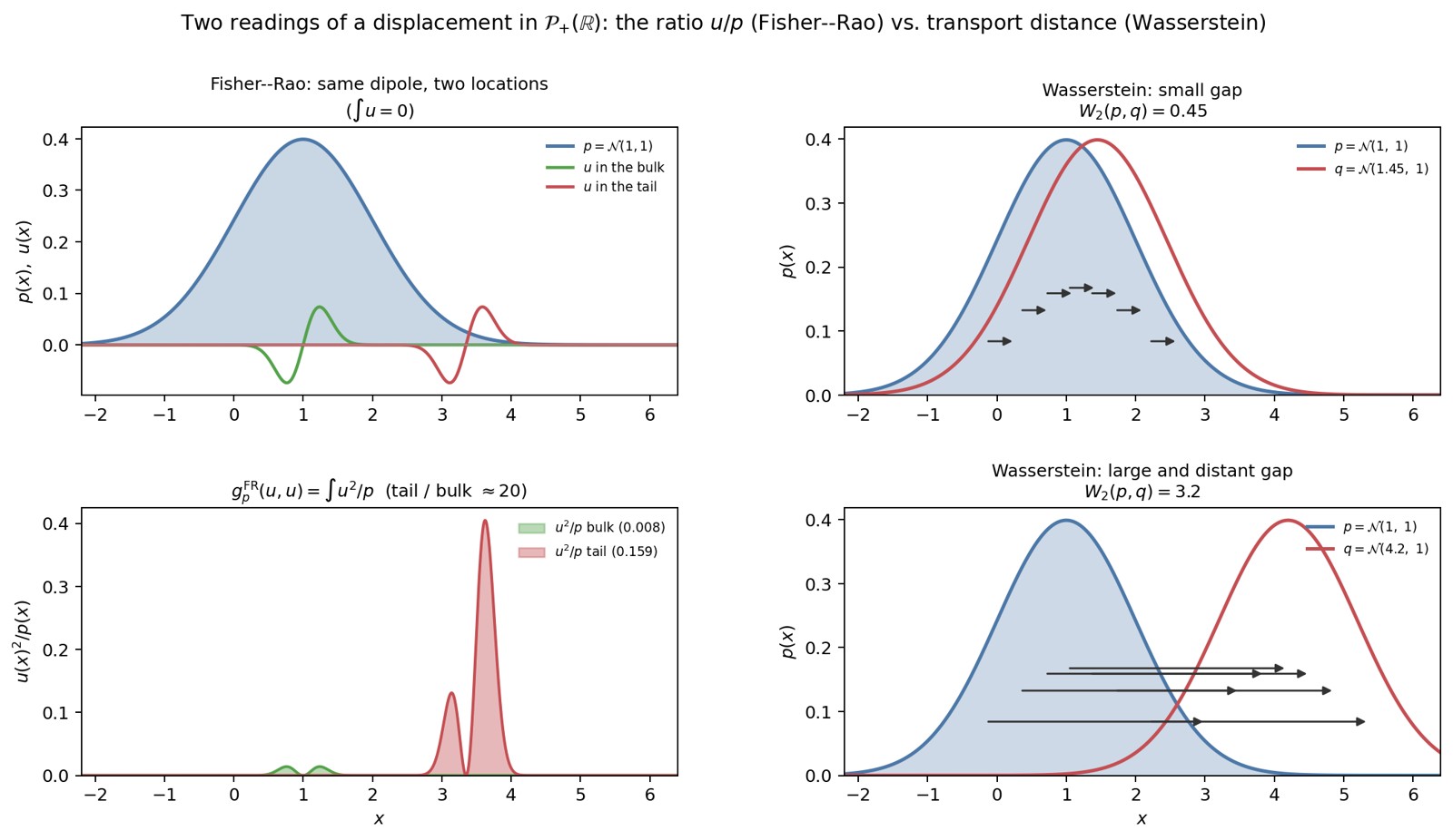
Figure 6. Two interpretations of a displacement in
.
On the left, Fisher–Rao: the same dipole
,
with
,
has a low cost at the centre of
and a high cost in the tail, where
is small. On the right, Wasserstein:
is translated first by a small displacement and then by a large one; the
cost is the length of the transport arrows.
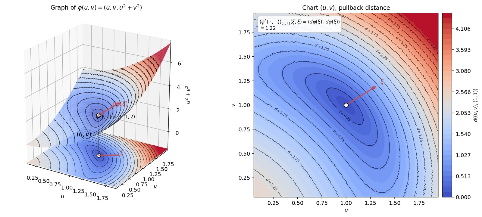
Figure 7. Graph of
in
,
coloured by a numerical approximation of the Riemannian distance to the
point
(geodesic shooting, Runge–Kutta 4), and the same function on the
parameter plane
.
The iso-contours on the graph can be read again in the chart: this is
the pullback. The arrow
in the plane is mapped to
;
by definition,
.
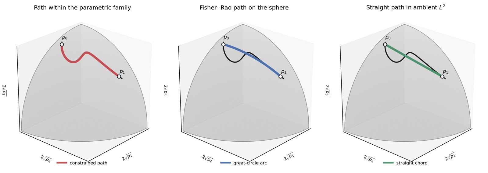
Figure 8. Three paths between the same two points under the
square-root embedding
.
The grey surface is the positive orthant of the sphere of radius
,
and the black curve is a parametric subfamily. Left: the red path
remains within the subfamily. Centre: the blue Fisher–Rao geodesic may
leave the subfamily but remains on the sphere. Right: the green straight
chord leaves the sphere and lies in the ambient
space of square-root coordinates. This last path represents the chordal,
or Hellinger, geometry and should not be confused with the ordinary
straight line between the original densities.
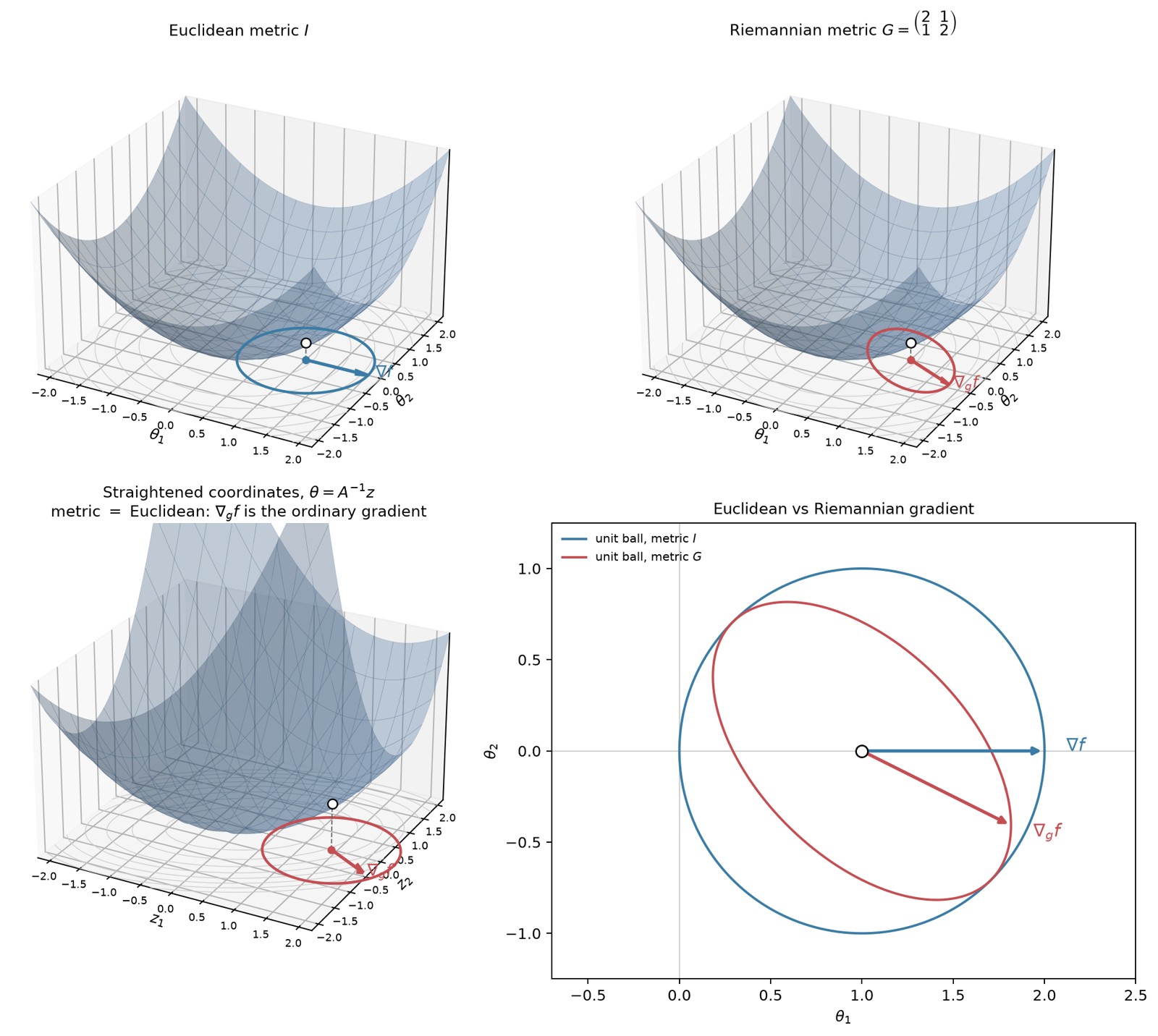
Figure 9. Geometric interpretation of the natural gradient in the
two-dimensional example. Top left: the Euclidean unit circle and the
Euclidean gradient on the graph of
.
Top right: the same graph with the Riemannian unit ellipse
and the Riemannian gradient. Bottom left: the coordinates
,
with
,
straighten the metric locally and turn the ellipse into a Euclidean unit
circle. Bottom right: direct comparison of the Euclidean and Riemannian
gradients in the original parameter coordinates.
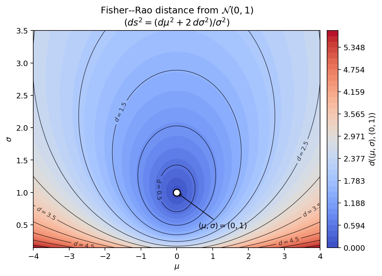
Figure 11. Fisher–Rao distance from
in the parameter plane
.
Blue-to-red colour map and level sets; the “circles” of the metric are
not Euclidean circles.
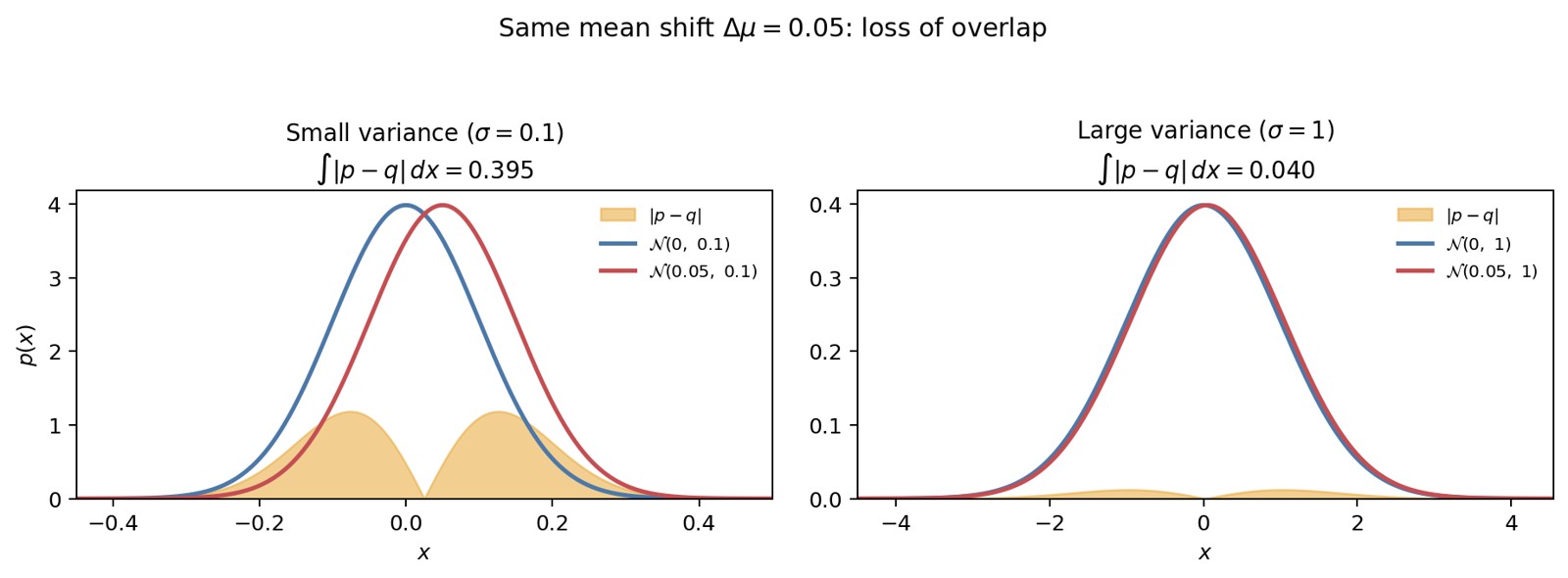
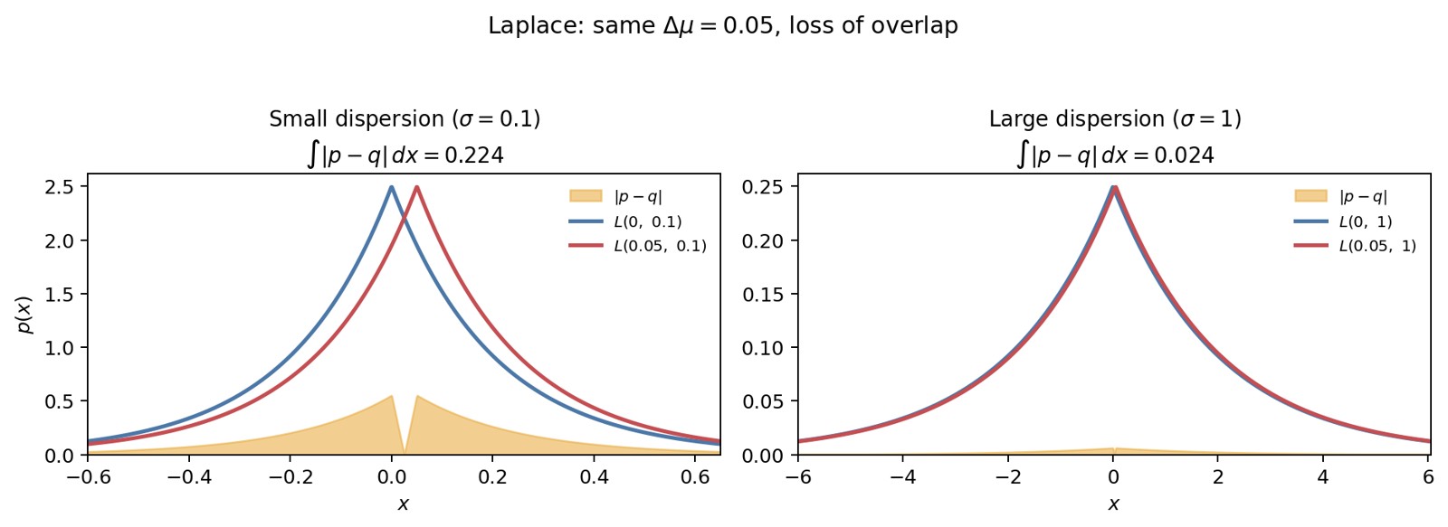
Figure 12. The same mean shift
.
On the left, with
,
the densities separate clearly
();
on the right, with
,
they remain almost indistinguishable
().
The orange area marks the loss of overlap.
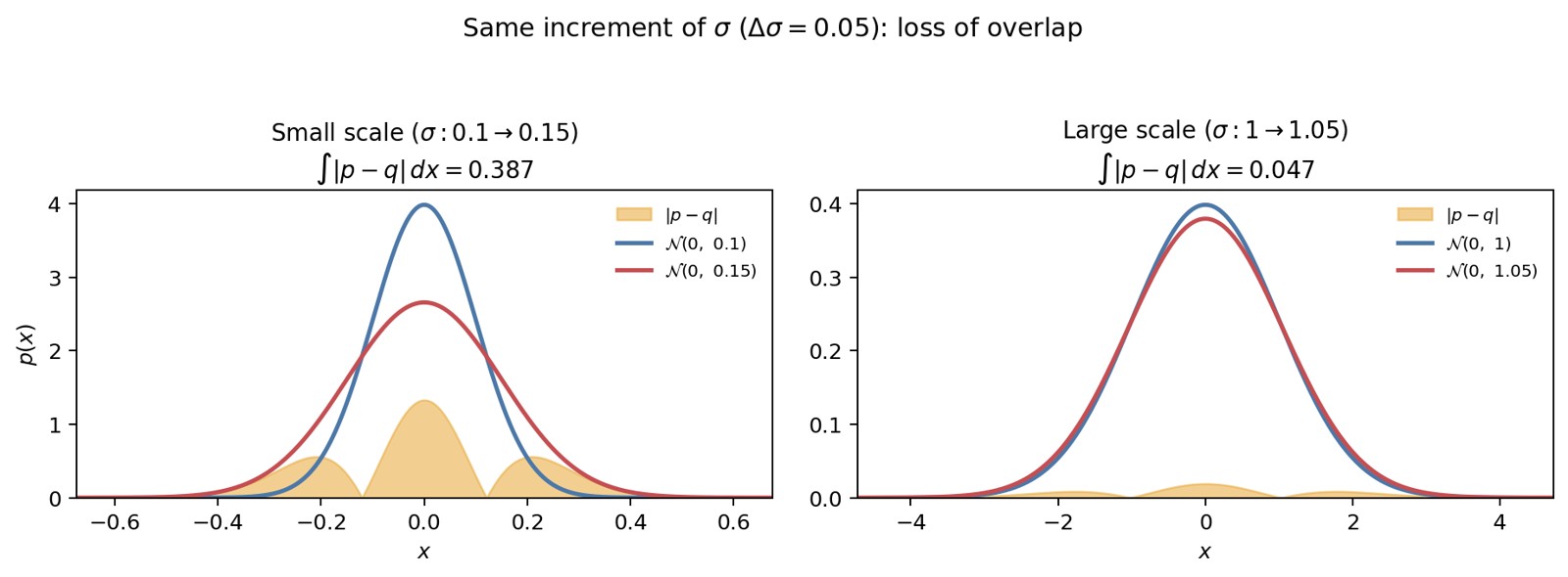
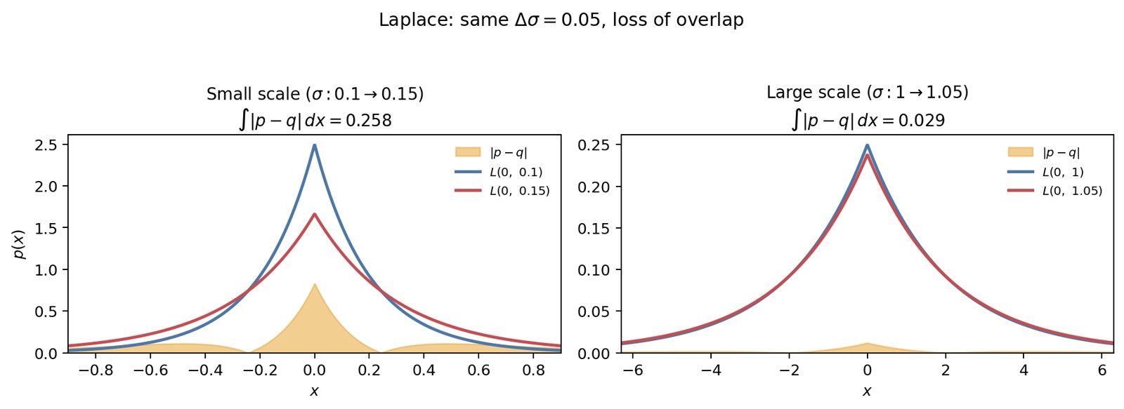
Figure 13. The same increase in standard deviation
.
On the left, from
to
,
the profile changes considerably; on the right, from
to
,
it barely changes. Once again, the cost depends on the current scale of
.
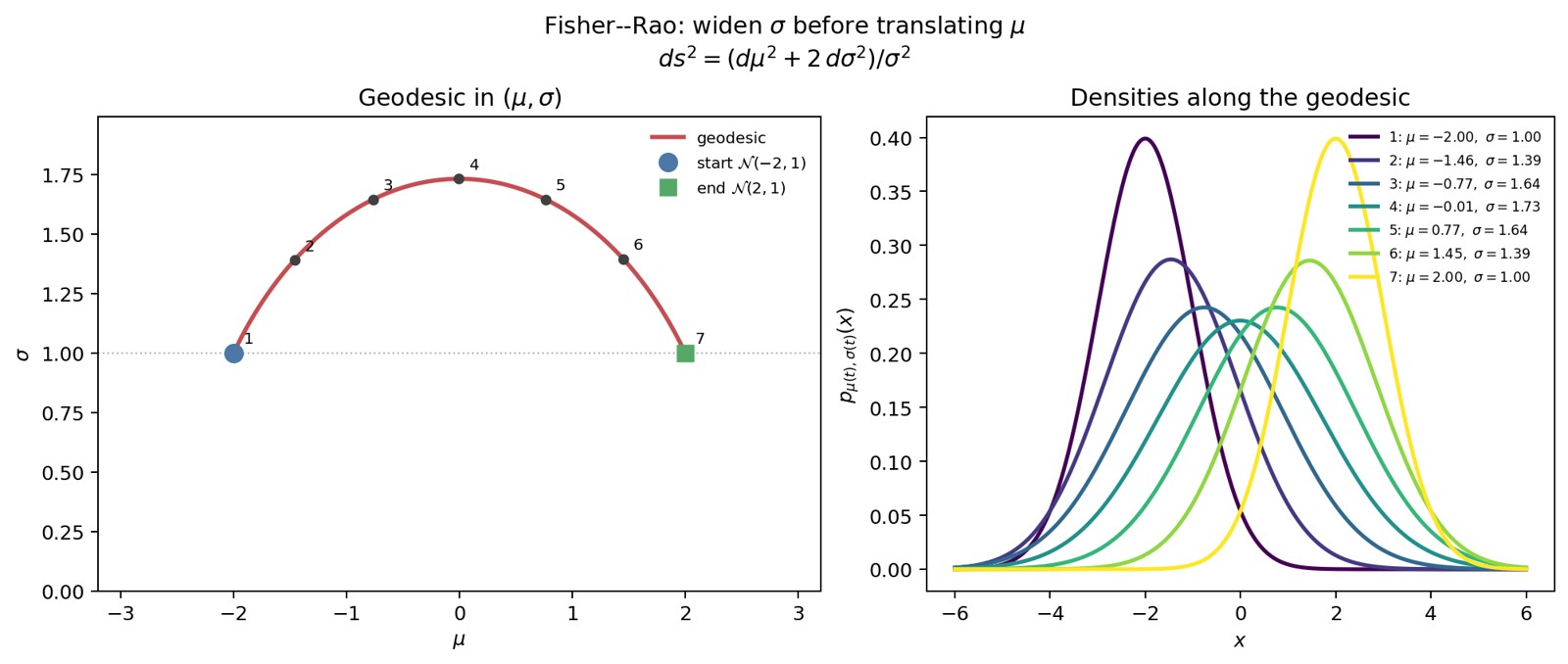
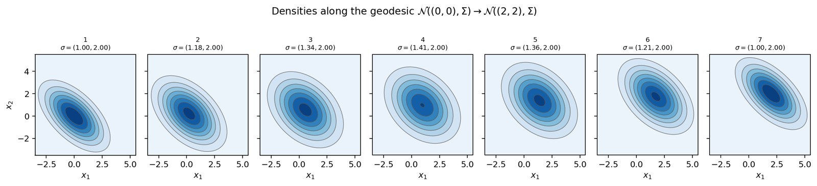
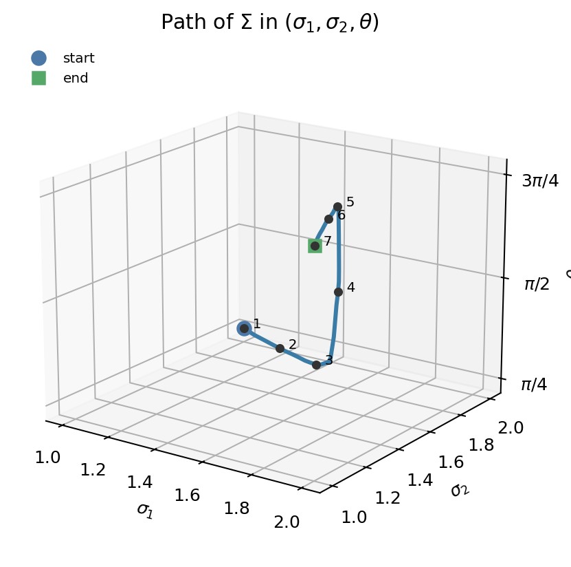
Figure 14. Fisher–Rao geodesic from
to
.
On the left, the arc in
;
on the right, the densities at the numbered points. We increase
before translating
.
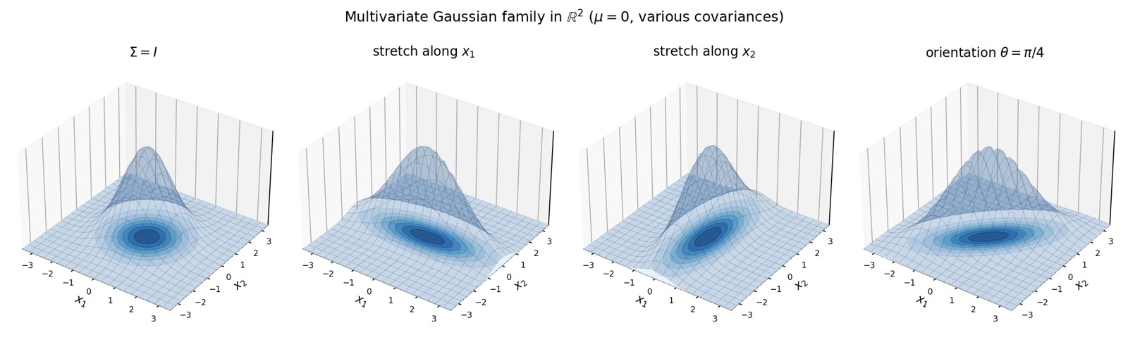
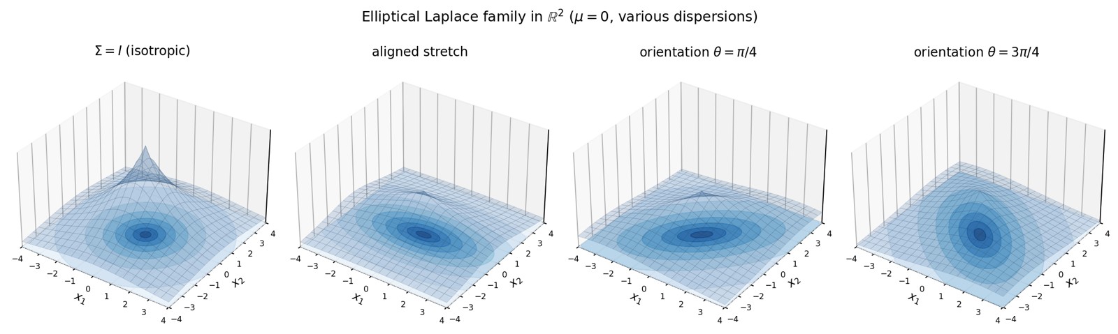
Figure 15. Four multivariate Gaussians in
,
centred at
.
From left to right:
,
elongation along
,
elongation along
,
then orientation
.
The surface represents the graph of
;
the curves on the base plane are the level sets of the
density.
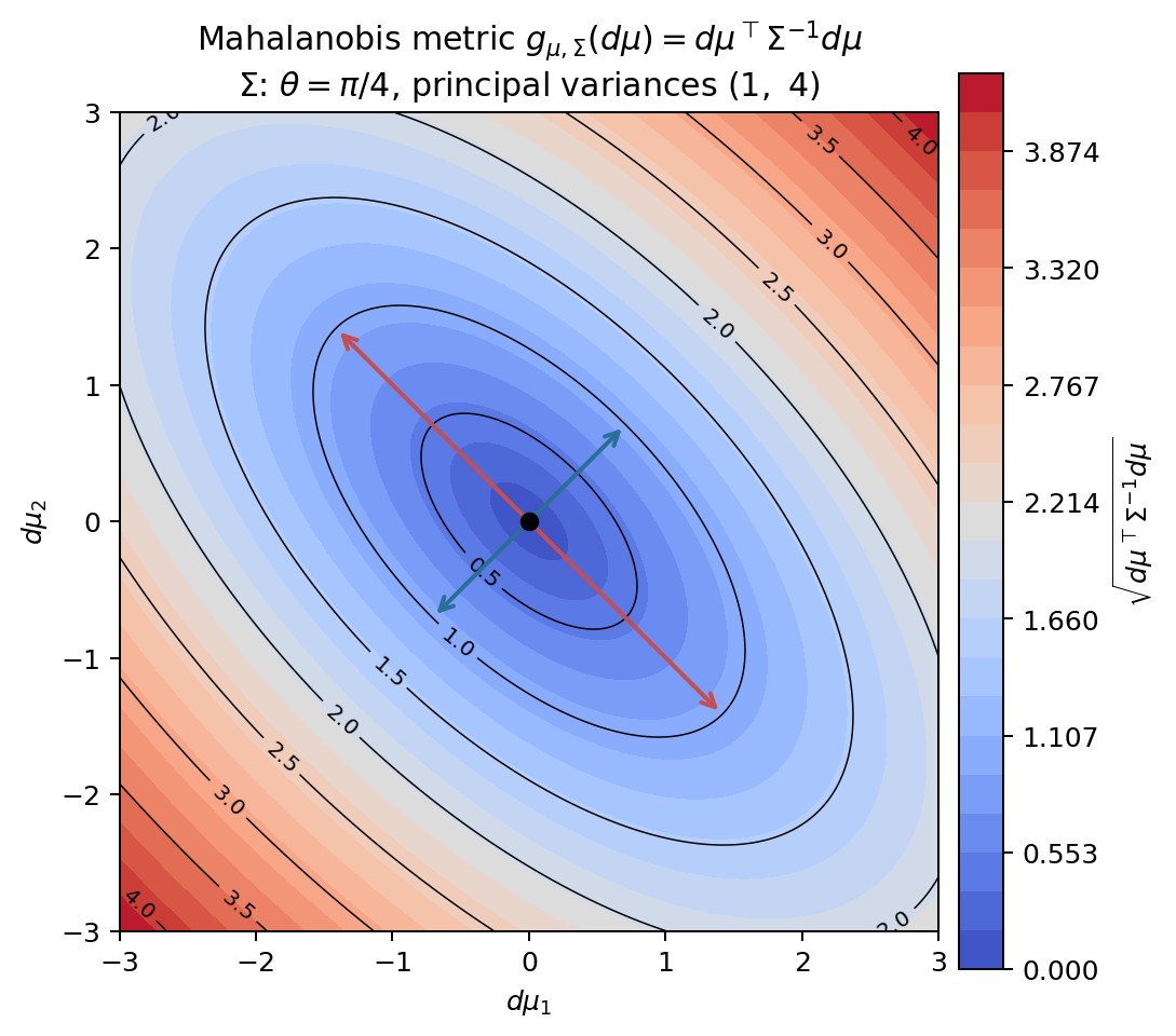
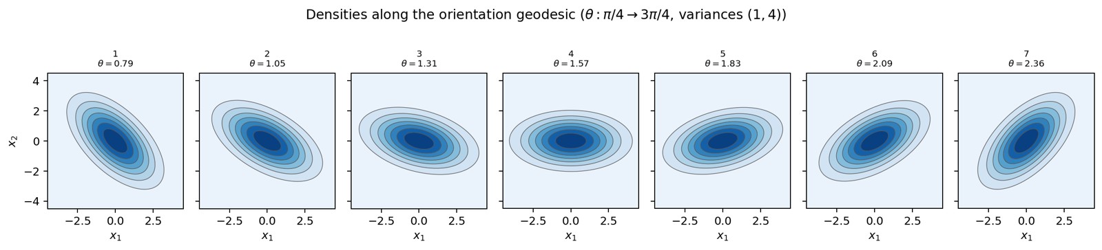
Figure 16. Metric
on mean displacements, at fixed
.
Here
has angle
and principal variances
.
The level sets are Mahalanobis ellipses; the arrows mark the principal
axes.
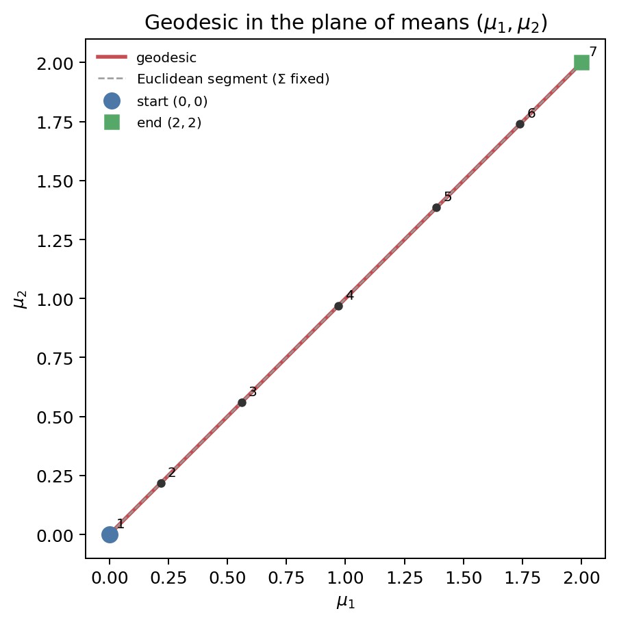
Figure 17. Numerical approximation of a Fisher–Rao geodesic from
to
,
projected onto the
plane, with
fixed at
.
The mean displacement follows the line segment; it is
that changes.
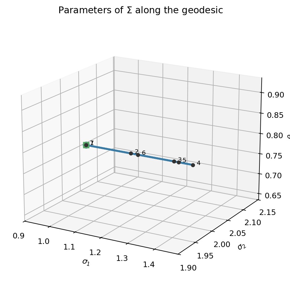
Figure 18. Parameters
of
along the same curve. The standard deviations move away from their
endpoint values in the middle of the path (spreading), then return to
them;
is constrained to
.
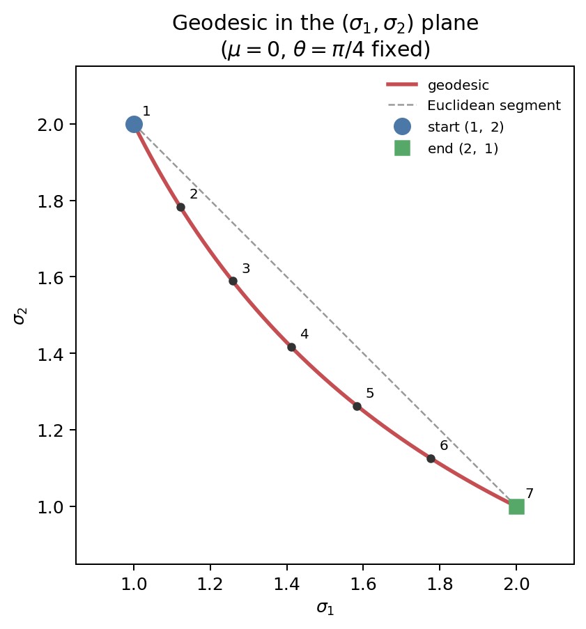
Figure 20. Fisher–Rao geodesic in the
plane, with
and
fixed. The path is a hyperbola (a straight line in logarithmic
coordinates), distinct from the Euclidean line segment.
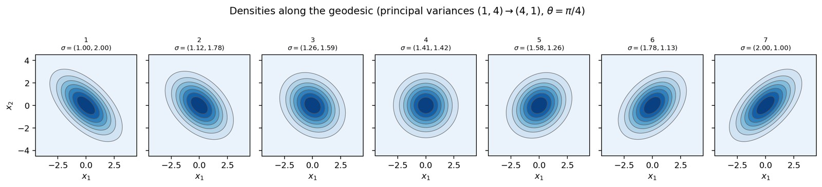
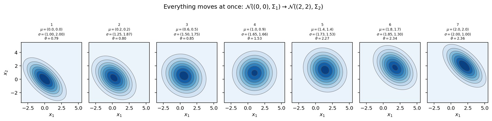
Figure 24. Numerical approximation of a Fisher–Rao geodesic between two
general bivariate Gaussians (discrete energy minimization). At each
step,
,
,
and
evolve simultaneously.
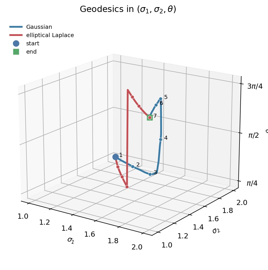
Figure 30. Numerical approximations of the Fisher–Rao geodesics between
the same endpoint parameters, projected into
.
Gaussian in blue, elliptical Laplace in red.
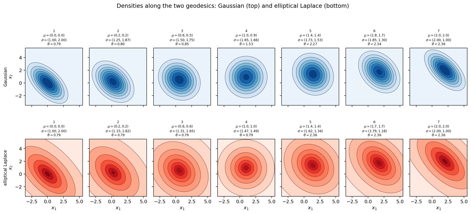
Figure 31. Evolution of the densities along the two numerical curves,
at the same seven stages: Gaussian on the top, elliptical Laplace on the
bottom. Each panel shows the values of
,
,
and
.
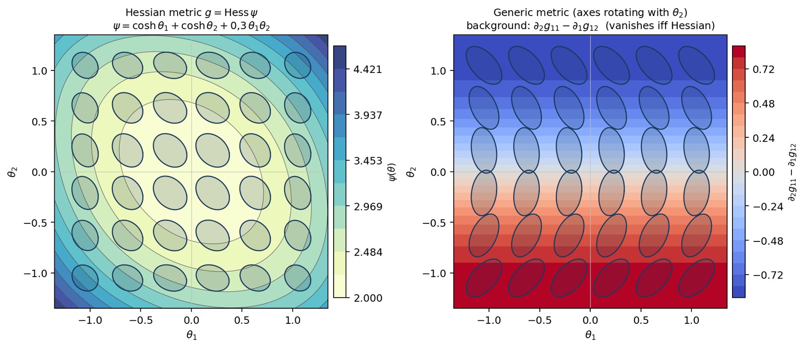
Figure 34. Circles of the metric in the
plane. On the left,
:
the background shows the level sets of
.
On the right, a field with fixed eigenvalues whose axes rotate with
;
the background,
,
is the Schwarz obstruction, which vanishes if and only if
is a Hessian metric.
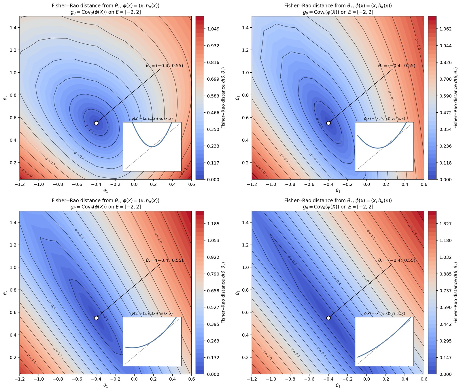
Figure 35. Progressive degeneration of the Fisher–Rao metric for a
linear Gibbs family. The panels show the Fisher–Rao distance from the
reference parameter
for
as
decreases from
towards
.
The metric is
For
,
traces a parabola: its two components are affinely independent and the
metric is positive definite. As
,
the image of
becomes increasingly close to the affine line
.
One eigenvalue of
then becomes small: the corresponding direction in parameter space
produces an almost constant variation of the energy and therefore hardly
changes the density. The progressive stretching of the iso-distance
contours makes this near-degeneracy visible. In the limit
,
the image is contained in a line, the parametrization becomes redundant,
and the Fisher–Rao metric loses rank.
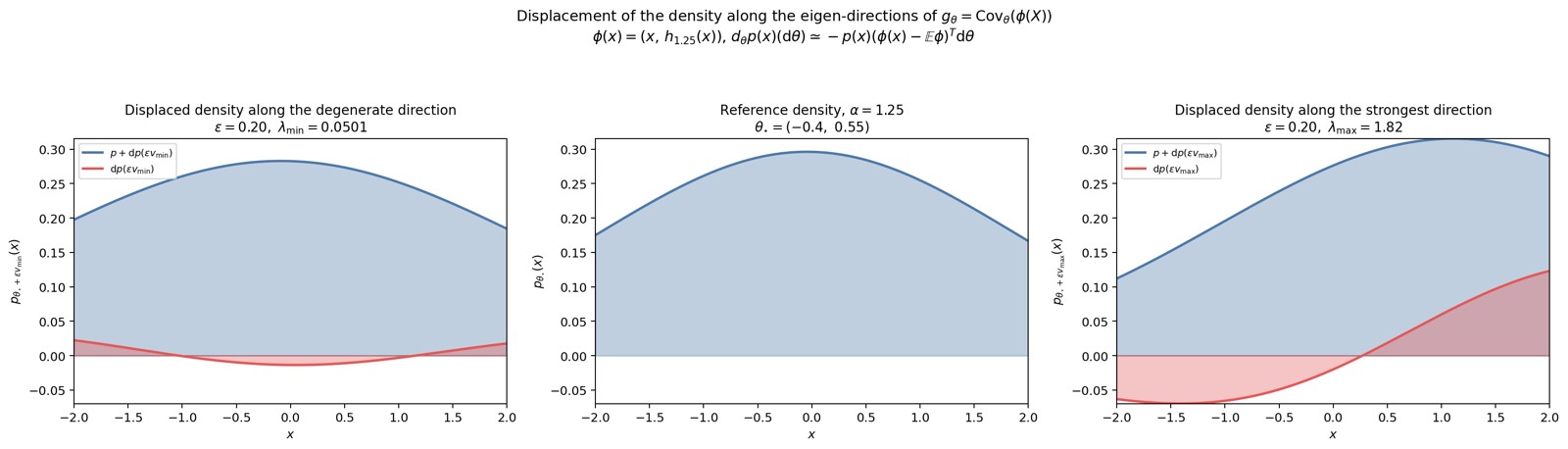
Figure 36. A step of the same Euclidean length
along each eigen-direction of the metric at
,
for
.
The middle panel shows the reference density
;
the side panels show the displaced density
in blue together with the displacement
in red. On the left, the step is taken along the direction of the
smallest eigenvalue: the displacement is weak, the density barely
changes. On the right, the same step is taken along the direction of the
largest eigenvalue: the displacement is much stronger and visibly
reshapes the density.
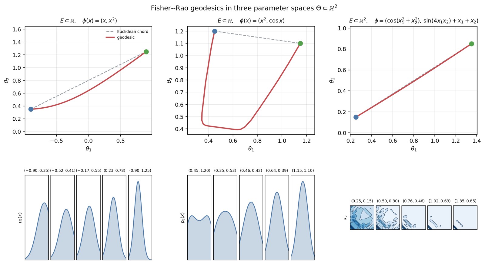
Figure 37. Numerical approximations of Fisher–Rao geodesics (discrete
energy) on three parameter spaces
,
the metric
being evaluated by a Riemann sum on a bounded window. The first two
families are defined on
,
the third on
.
Departure in blue, arrival in green; densities at the intermediate
points.
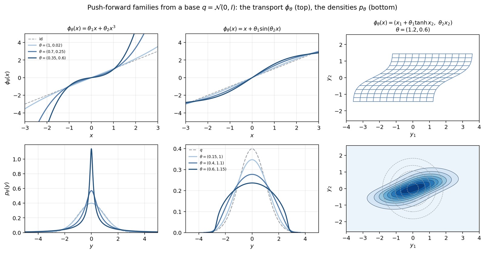
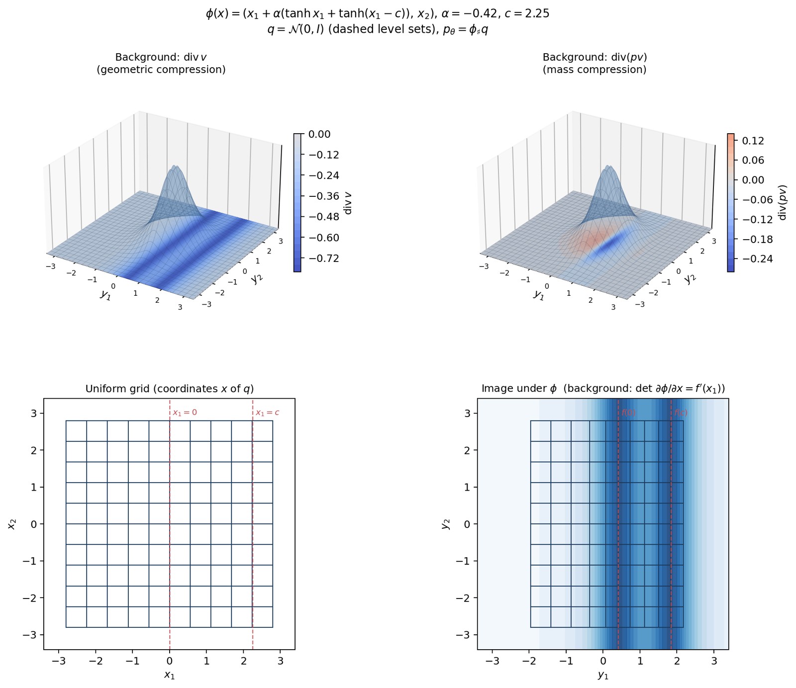
Figure 39. Three push-forward families of a standard Gaussian base. At
the top, the transport
itself: the curves
for the two one-dimensional examples (the identity in dashes), and the
image of a grid for the two-dimensional example. At the bottom, the
resulting densities
,
with the base
in dashes.
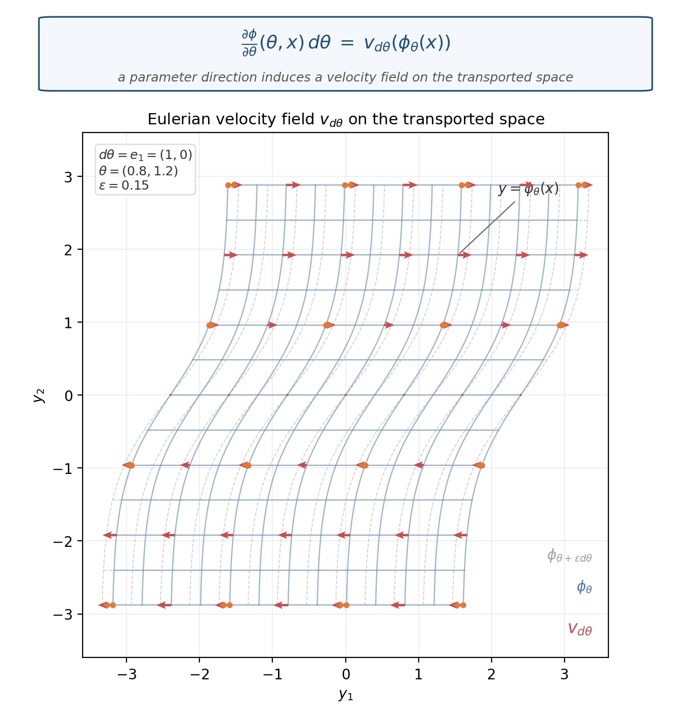
Figure 40. Eulerian velocity field induced by a parameter direction.
Transport
at
,
with
.
Solid: the grid transported by
.
Dashed: the same grid after
,
.
Red arrows:
at
,
computed from the initial point
.
A direction in
becomes a vector field on
.
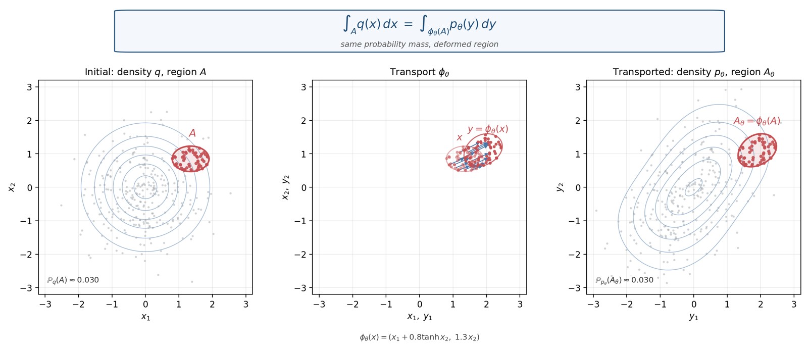
Figure 41. Conservation of probability under a push-forward. Base
and transport
,
with
.
Left: density
,
region
,
and particles from the base (in red those of
).
Middle: the same particles of
mapped by
.
Right: density
,
transported region
,
and the same particles after transport. The probability mass of the
material region is unchanged.
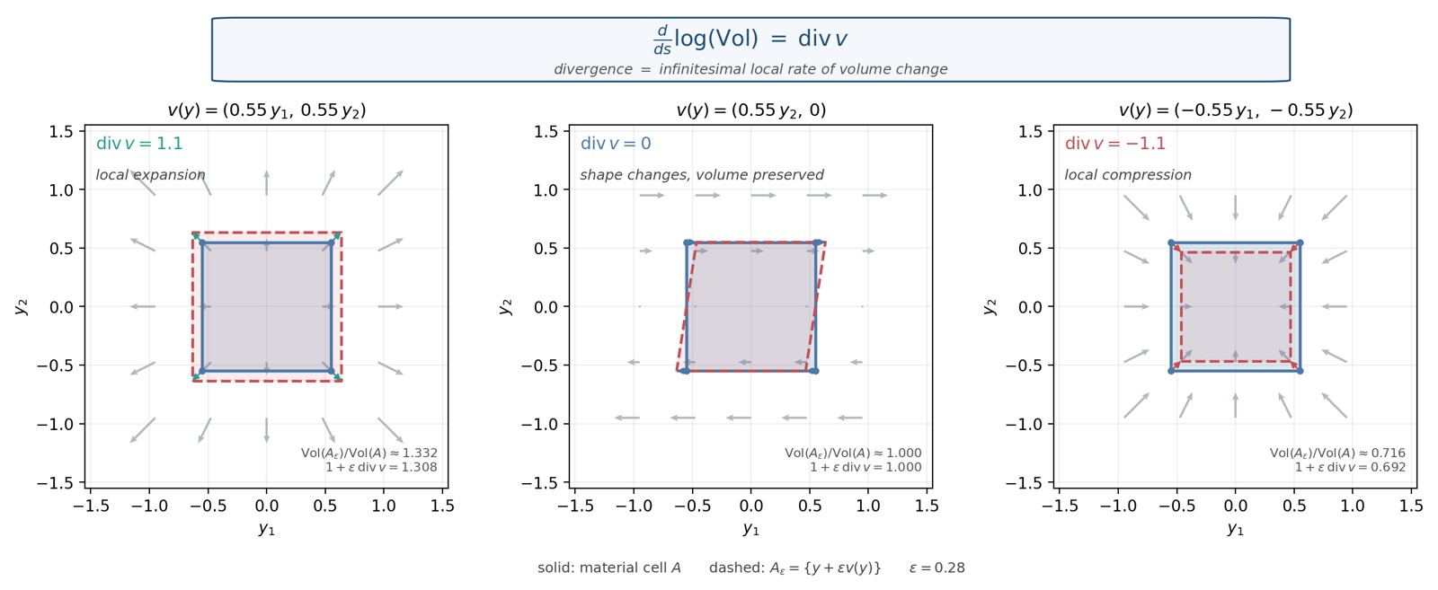
Figure 42. Divergence as infinitesimal local rate of volume change. The
same material cell
(solid) is deformed by
(dashed),
.
Left: radial expansion
,
.
Middle: shear
,
:
the cell becomes a parallelogram, the area is unchanged. Right: radial
compression
,
.
The numerical ratios
match
to first order.
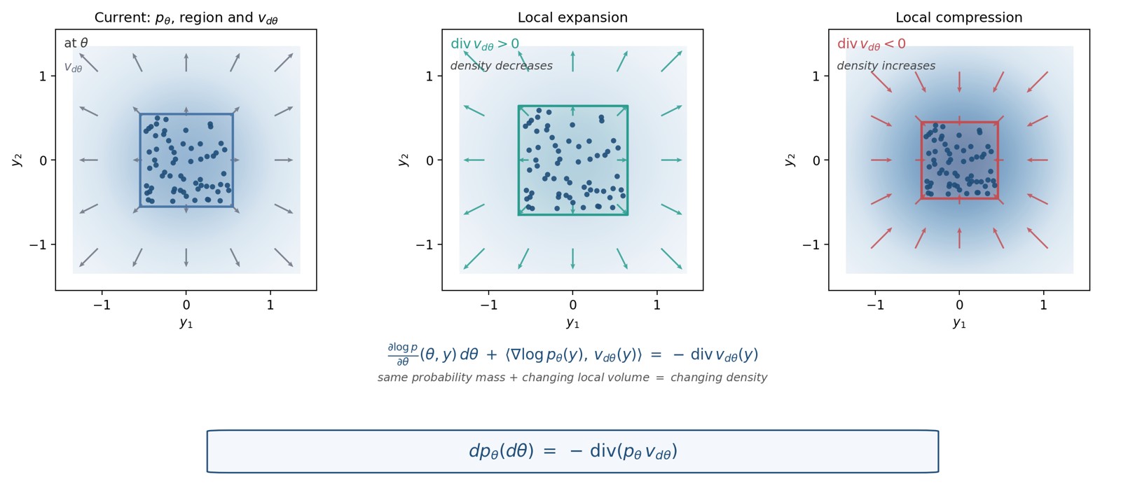
Figure 43. From volume change to density change, under conservation of
probability. Left: a material cell at
,
with local shading of
,
particles for the probability mass, and arrows of
.
Middle: local expansion
:
the same particles occupy a larger cell, the density decreases. Right:
local compression
:
the same particles occupy a smaller cell, the density increases. The
particle count is identical in the three panels.
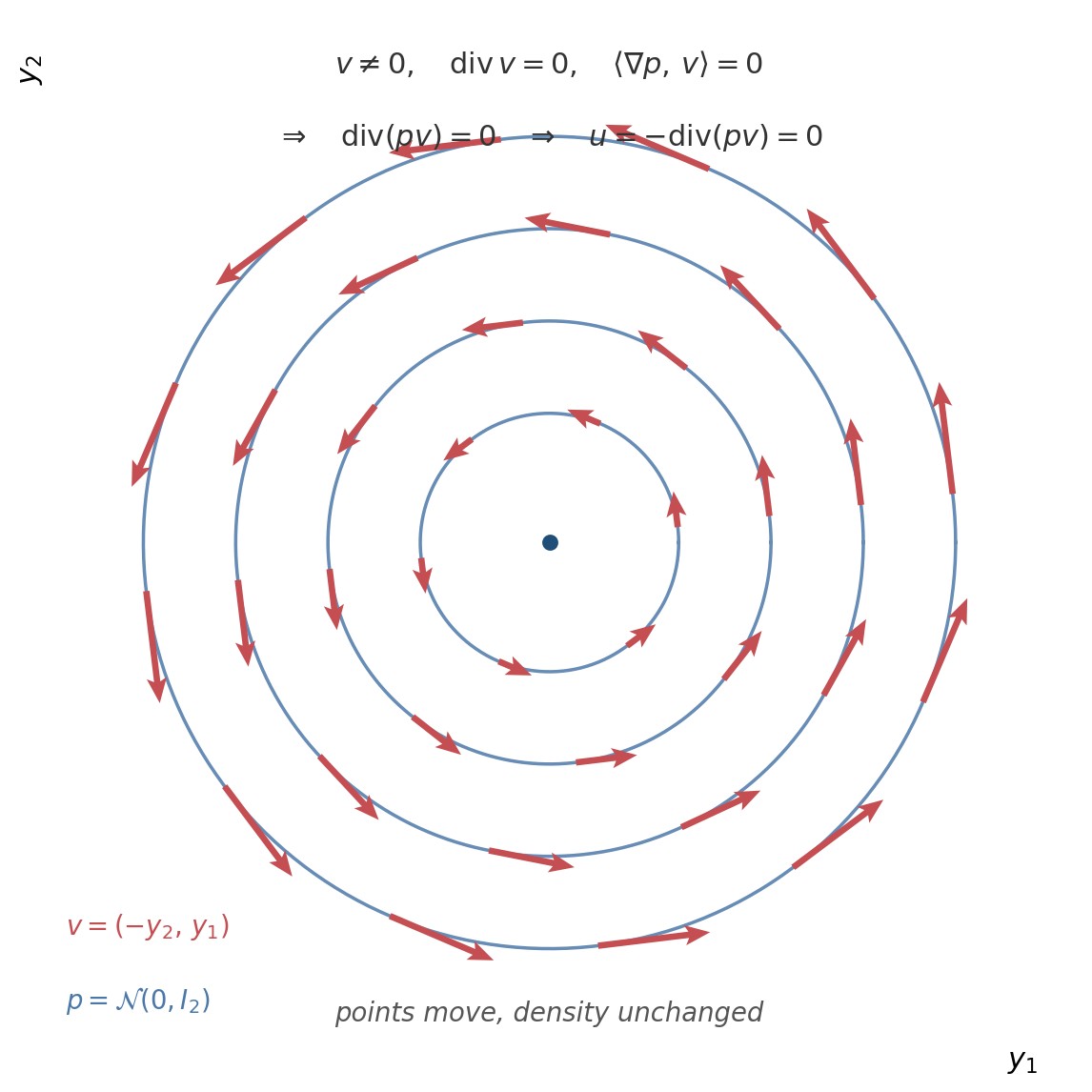
Figure 44. A nonzero velocity field invisible to Fisher–Rao. Level sets
of
and the rotational field
.
The arrows are tangent to the contours:
and
,
so
and
.
The points move, the density does not change.
Figure 45. Transport
of a standard Gaussian,
,
.
At the top, the same density
;
the floor is
on the left and
on the right. At the bottom, the uniform grid in the coordinates of
,
then its image by
.
The two squeezes read on the grid as clearly as each other; Fisher–Rao
keeps only the one in the bulk.
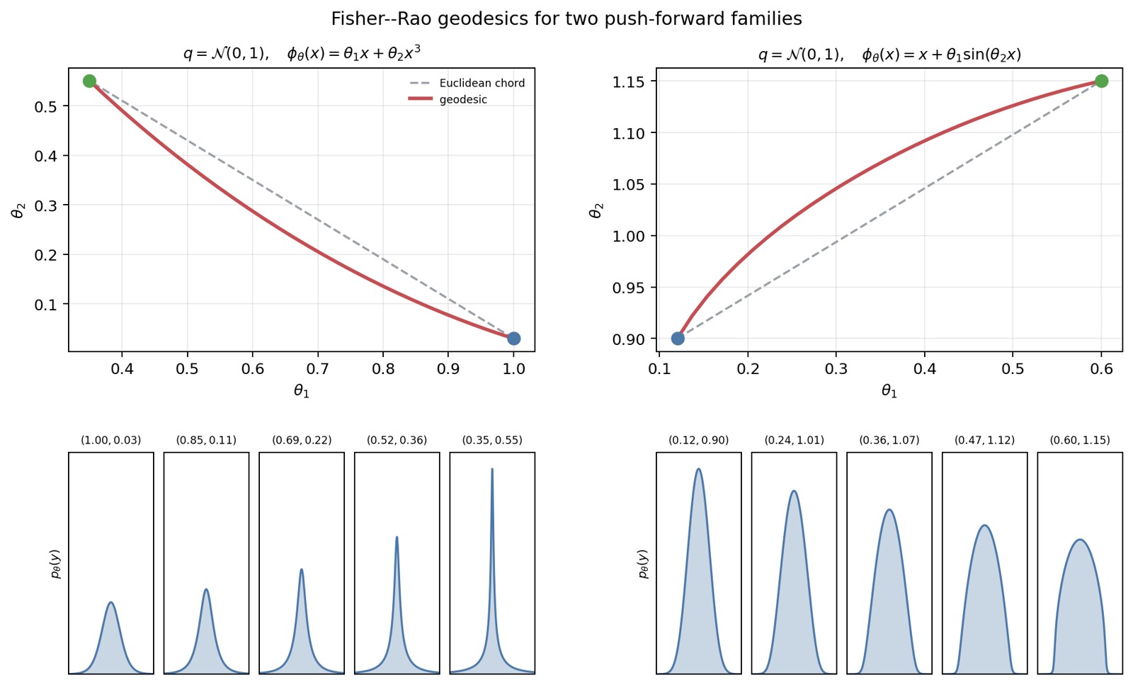
Figure 46. Numerical approximations of Fisher–Rao geodesics for two
push-forward families,
(discrete energy, metric by quadrature on the base). At the top the path
in
(in red), compared with the Euclidean chord (in dashes); at the bottom
the densities
along the path, with
in the title.
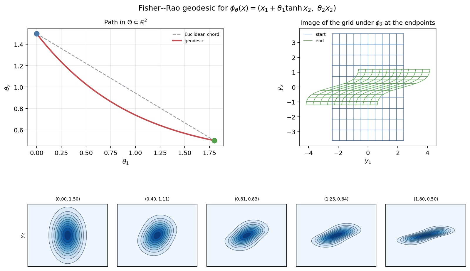
Figure 47. Numerical approximation of a Fisher–Rao geodesic for the
two-dimensional transport
,
base
.
At the top left the path in
and the Euclidean chord; at the top right the image of a grid by
at the two endpoints, which shows the non-affine shear; at the bottom
the densities along the path, with
in the title.